Time Series Analysis – A Gentle Introduction

Time series data contains a column of values (e.g sales, costs) and a column of even time intervals (eg. days or months). Time series analysis concerns understanding the relationship between those values (sales, costs etc.) and time (prior period values). Time series analysis automatically finds correlations between current and prior periods and uses those relationships to forecast future periods.

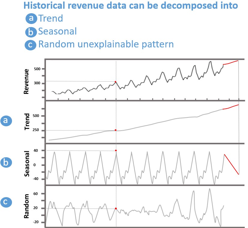
The main idea: we can decompose a time series data set into trend and seasonal components which separately are easier to forecast.

There are two types of correlations (relationships) that can be discovered:

• Trend relationships: for example, the data can show a long term rising trend, decreasing trend, or no trend.
• Seasonal relationships: for example, December sales are the holiday period and can be a good predictor for next Decembers sales

There are several questions machine learning can help answer:

• Is it a number
• Is it a category
• Is it a group

Forecasting distinctly deals with predicting a number. Forecasting almost always involves time series data. Examples of time series data include weekly actual sales of a computer mouse product from 2013 to 2016, or daily exchange rates between the EURO and US dollar. In both case the data set has two columns: time and value.

There are two important characteristics of time series data. 1. Data is ordered by time. In many other data sets discussed in this book, the order of the rows is not important. However, for time series data order matters and the order is defined by the column labeled time. Another important characteristic of time series data is that intervals between time stamps is equally spaced. A data set of annual sales that has weekly data for 5 months and then monthly data for the remaining 7 months will cause problems for forecasting.

There are two classes of models most commonly used for forecasting

1. Time Series Analysis and
2. Regression-based models

Time Series Analysis

As with most statistical analysis, correlation is a necessary condition for modeling. With Time Series Analysis there is a special kind of correlation that the algorithm seeks, namely, correlation of a specific time-stamped value with a previous time-stamped value. In other words, the algorithm seeks to understand if today’s sales are correlated with yesterday’s sales, or yesterday and day before’s sales, or last Novembers sales. This correlation has a special name: Auto-correlation. 3. Time series observations are dependent. The reader may be familiar that the assumptions of many machine learning models is that the data are independent and identically distributed (iid).

Time Series Models

Three types of Time Series Models are most commonly used

1. ARIMA (Autoregressive Moving Average)
2. STL (Seasonal Decomposition of Time Series by Loess)
3. ETS (Exponential Smoothing)

Before describing these models, it is useful to discuss what information prior-period sales can reveal.

To do that we will look at the follow fictitious plot of historical sales of a product.

1. Trend.

Time series analysis can reveal if there is a long term trend, either declining or increasing. In the above chart it is evident that over the period covered on the chart there is a long-term increasing trend.

1. Seasonality

Time Series analysis can reveal if there are seasonal patterns in the data. For example, for certain consumer products, Black Friday sales may always spike suggesting that this year’s week 4 of November sales is correlated with last years and pervious years week 4 November sales.

 

Trend	Seasonality	Example	Notes
Yes	No		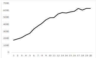The time series data shows a long term year-over-year increasing trend. Example: number of internet users
No	Yes		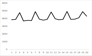The time series data shows an evenly-spaced seasonal pattern. Example: a company’s sales spike every quarter at the end of the fiscal quarter.
Yes	Yes		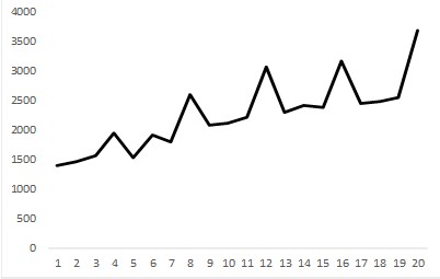The time series data shows both a long term trend as well as a regularly spaced seasonal pattern. Example: annual sales of air conditioners spike in the summer.
No	No		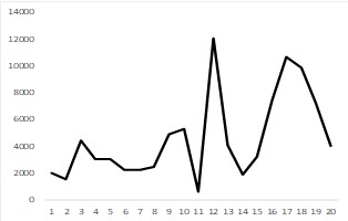The time series data shows no clear trend nor seasonal pattern. Note: time series methods are not suitable for this data set.

Forecasting the Constituent Parts

The main idea is that decomposing a time series into its constituent parts makes it easier to forecast the constituent parts and re-aggregate the parts into a forecast. There are models that’s sum the parts (known as additive models), that multiply the parts (known as multiplicative models) and other variations. The intuition may be apparent from the following figure. Imagine forecasting the next period for the trend just the trend line. It is pretty clear that the next point will be somewhat higher.  Imagine forecasting the next period for the seasonal component. It seems clear that the next period will be lower. Once the time series model has forecast the next period values for the trend and seasonal components, the algorithm aggregates the forecasted points to get a new forecasted value.