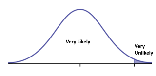
A friend recently asked me what is a P-value. I have previously described P-values in presentations but his question prompted me to write a blog post on it. If statistics has a reputation for being non-intuitive, I will admit that P-values is one of the main culprits. According to Wikipedia, “the P-value is the probability of obtaining a test statistic at least as extreme as the one that was actually observed, assuming that the null hypothesis is true.” Huh? That is as difficult to understand as some of the interviews here in this fivethirtyeight.com article – Not Even Scientists Can Easily Explain P-values..
My friend just wanted to know conceptually what is a P-value.
tl;dr
P-values are measures that help us decide if our data is statistically significant or not.
1 liner: A P-value measures whether we can infer that our statistic is statistically significant or whether it could be due to chance (i.e. not statistically significant)
3 liner: In statistics we often want to make inferences about a group, such as inferring that that the average weight of group A is larger than the average weight of group B. Our statistical estimates may indicate there is a difference, but we have to account for the possibility that the difference we observe could be due to random chance and not something else. P-values measure whether we can infer that our statistic (the difference) is statistically significant, or whether it could be due to random chance.
2 Examples
The main idea is that if you were 100% certain that there is no difference between two groups, it is still possible that you may see a difference when you sample from those two groups. That is because of chance. Let’s look at some simple examples.
Example 1: you have a coin that has been evaluated by the International Institute of Fair Coins and tested to be fair. You know that there is a 50% chance of landing on tails and 50% chance of landing on heads. You flip the fair coin 10 times: 7 times it lands heads, 3 times it lands tails. Oh my, there is a difference. But it has already been evaluated by the International Institute of Fair Coins and confirmed to be fair. The difference observed is due to chance.
Example 2: You have an idea for a fitness app. Before developing the app you want to understand the following:
Is there a difference between the average daily steps of people living in a city and the average number of steps of people living in the suburbs.
You have defined the inference you want to make. The inference is about whether these two groups are different. Now you collect your data and analyze it:
- You randomly select 500 people from the city and 500 people from the suburbs
- You collect the average number of daily steps in each group
- You calculate the difference
| People who live in | Average Daily Steps |
| City | 9000 |
| Suburban | 7500 |
| Difference | 1500 |
1500 is a big difference. That difference could be due to some phenomenon such as more people have cars in the suburbs. Or it could be due to chance, such as when you sampled it had been raining in the suburbs causing people to use their car.
Data example 1: The Difference is Statistically Significant
Since these are samples, and we cannot say with 100% precision that the difference is the true value. As shown in the coin tossing example, it is possible that there is no difference because the data you observed is due to chance.
You declare 5% as your minimum bar for inferring significance. This means you must calculate a 95% confidence interval and your data shows:
| Mean Daily Steps | 95% Confidence Interval | Low | High | |
| City | 9000 | +/- 600 | 8400 | 9600 |
| Suburban | 7500 | +/- 500 | 7000 | 8000 |
How do we interpret this?
- We are 95% confident that the true average of the City data lies somewhere between 8400 and 9600
- We are 95% confident that the true average of the Suburban data lies somewhere between 7000 and 8000
Since we want to know if difference in averages is significant, we need to look at all the possible outcomes.
| Mean Daily Steps | 95% Confidence Interval | Low | High | High minus low | Low minus High | |
| City | 9000 | +/-600 | 8400 | 9600 | 9600 | 8400 |
| Suburban | 7500 | +/-500 | 7000 | 8000 | 7000 | 8000 |
| Difference | 1500 | 2600 | 400 |
The difference could be 1500, it could be 2600, or it could be 400. In all cases there is a difference. There is no case where the difference is zero.
Here is what the confidence intervals look like on a chart. Note there is no overlap of the two ranges.
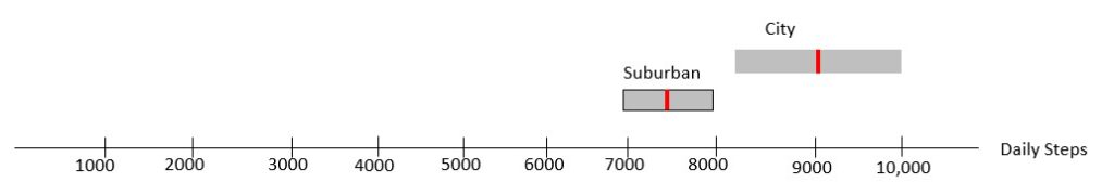
We can conclude that the difference in average daily steps between peple who live in the city and people who live in suburbs is statistically significant.
Data example 2: The Difference is Not Statistically Significant
What if our data looked like this?
| Mean Daily Steps | 95% Confidence Interval | Low | High | High minus Low | Low minus High | |
| City | 9000 | +/-600 | 8400 | 9600 | 9600 | 8400 |
| Suburban | 8000 | +/-500 | 7500 | 8500 | 7500 | 8500 |
| Difference | 1000 | 2100 | -100 |
1000 is a pretty big difference. But we want to know if the difference is significant so we have to look at all the possibilities. As we did in the previous example, let’s look at all the possible outcomes. The difference could be 1000, it could be 2100, or it could be -100.
Negative 100, what does that mean? That means there is a possibility that if the if the City average was on the low side of the of confidence interval, and the Suburban average was on the high side of the confidence interval, the difference could be equal to zero. For example:
City average could be 8450. Suburban average could be 8450 8450 – 8450 = 0
A difference that equals zero is another way of saying that they are the same.
Thus, we must infer that the difference observed is not statistically significant.
Visually we see the two lines overlap which indicates that there is a possibility that the averages are not different.